Course
DSP from Scratch
How a computer listens, measures and filters. The course starts with one question, what is a digital signal, and builds one idea at a time until you can design a filter and read a spectrum.
- 6 lessons out now
- 116 planned
- 9 parts
Part 1
Foundations
Samples, sine waves, aliasing, the impulse response, convolution and the frequency response.
6 lessons6 out
- 1
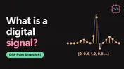 What Is a Digital Signal? Sampling and Sample RateHow a sound, a heartbeat or a video becomes a list of numbers.
- 2
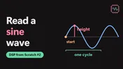 Amplitude, Frequency and Phase: How to Read a Sine WaveThe three numbers that describe any sine wave.
- 3
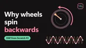 Why Wheels Spin Backwards on Video: Spectrum, Aliasing and NyquistSample too slowly and a fast signal dresses up as a slow one.
- 4
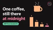 How Much Coffee Is Still in You at Midnight? The Impulse ResponseTap a system once and watch how it answers.
- 5
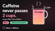 Convolution Explained Simply: Flip, Slide, Multiply, AddThirty coffees, and still never two cups.
- 6
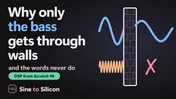 Frequency Response Explained Simply: Gain, Phase and FiltersWhy only the bass gets through the wall.
Part 2
The tools and the rules a system follows
Complex numbers as arrows, then the rules a system follows: linearity, time invariance, causality and stability.
12 lessons
See the 12 lessons planned
- 7Tools: a complex number is an arrow
- 8Tools: multiplying arrows: lengths multiply, angles add; polar form, conjugate
- 9Tools: Euler's formula, e^(jθ) as a spinning arrow; a cosine is two arrows
- 10Digital frequency: cycles and radians per sample, why ω stops at π
- 11Linearity: the scale-and-add test
- 12Time invariance: the delay test
- 13Causality: no peeking at the future
- 14Stability: bounded in, bounded out (sum of |h|)
- 15Difference equations: a filter as a recipe
- 16Block diagrams: adders, multipliers and the delay box z⁻¹
- 17FIR and IIR: filters without and with feedback
- 18Solve with me: system properties
Part 3
The frequency domain
How much of each frequency a signal holds, ideal and real filters, linear phase and group delay.
15 lessons
See the 15 lessons planned
- 19The DTFT: measuring how much of each frequency (analysis equation)
- 20Building the signal back: the inverse DTFT (synthesis equation)
- 21Why a digital spectrum repeats every 2π
- 22Frequency response, properly: e^(jωn) in, H(ω)e^(jωn) out
- 23Tools: decibels, and reading magnitude and phase plots
- 24The moving-average filter of any length, in frequency
- 25Ideal filters: low-pass, high-pass, band-pass, band-stop
- 26Why the ideal filter can't be built (infinite, non-causal)
- 27Real filters: passband ripple, stopband, transition band
- 28FIR or IIR? The trade-off, on a noisy signal
- 29Linear phase: every frequency delayed by the same amount
- 30Proving it: symmetric taps (the Type I derivation)
- 31Group delay
- 32What non-linear phase does to a signal, and forward-backward filtering
- 33Solve with me: frequency response
Part 4
The z-transform
Poles, zeros and the region of convergence: reading a whole system from one map.
19 lessons
See the 19 lessons planned
- 34Why engineers draw poles and zeros (a recipe you can't read by eye)
- 35Tools: the geometric series and when it adds up
- 36The z-transform, and why a delay is written z⁻¹
- 37When the sum converges: the region of convergence
- 38The z-plane, the unit circle and the DTFT
- 39Building the table of z-transform pairs
- 40Causal, anti-causal and two-sided signals
- 41Same X(z), different signals: the ROC decides
- 42Properties that save work (shift, convolution → multiplication)
- 43Rational transforms: poles, zeros and the pole-zero plot
- 44Tools: partial fractions
- 45Getting x(n) back: the inverse z-transform
- 46A double pole: the step convolved with itself
- 47The system function: difference equations become algebra
- 48Where a pole sits decides what the response does (real poles)
- 49Complex pole pairs: ringing that fades or grows
- 50Stability: poles inside the unit circle, ROC contains it
- 51Solve with me: transforms and ROC
- 52Solve with me: inverse and stability
Part 5
Poles, zeros and the frequency response
Walk round the unit circle and watch the frequency response take shape.
7 lessons
See the 7 lessons planned
- 53From H(z) to H(ω): put z on the unit circle
- 54Walk round the unit circle to see the response
- 55Gain is a ratio of distances
- 56Phase from the angles to poles and zeros
- 57The moving average puts its zeros evenly round the circle
- 58A zero's angle tells you which frequency disappears
- 59Solve with me: sketching responses from pole-zero plots
Part 6
FIR design by windows
From the ideal low-pass to a filter you can build, one window at a time.
17 lessons
See the 17 lessons planned
- 60The ideal low-pass becomes a sinc (the inverse DTFT at work)
- 61Keep M samples and move their centre to the middle
- 62What cutting does: ripples at the edge
- 63A window's spectrum: the main lobe sets the transition
- 64Sidelobes and the −13 dB problem
- 65Gentler windows: Hann, Hamming, Blackman
- 66Choose the window for ripple, then the length for transition
- 67Specifications in dB and in linear units
- 68A low-pass design, step by step
- 69Same design, four windows: what changes
- 70High-pass by subtracting from an all-pass
- 71Band-pass and band-stop from low-passes
- 72Symmetric taps: a delay times a real amplitude
- 73Better attenuation costs taps and delay; pros and cons of windows
- 74Equiripple: spread the error to shrink its worst peak
- 75Solve with me: FIR low-pass design
- 76Solve with me: FIR high-pass and band-pass
Part 7
IIR design
Filters with feedback: single poles, notches, combs, Butterworth and the bilinear transform.
17 lessons
See the 17 lessons planned
- 77One pole and one zero make a low-pass
- 78The 3 dB point: a quadratic for α
- 79Which root? α and stability; the "linear" phase myth
- 80Move the zero to z = 1 for a high-pass
- 81Band-pass: a complex-conjugate pair of poles
- 82Pole radius sets the bandwidth
- 83The notch: zeros on the unit circle
- 84Designing from hertz, and what the FIR equivalent costs
- 85Cascade identical sections for a sharper edge
- 86Tools: the nth roots, evenly round the circle
- 87The comb filter: replace each delay by L delays
- 88Tools: analogue filters and the s-plane
- 89The Butterworth prototype: maximally flat
- 90The bilinear transform and frequency warping
- 91A complete bilinear design in hertz, to the difference equation
- 92Solve with me: first- and second-order IIR
- 93Solve with me: bilinear design
Part 8
The DFT and the FFT
The spectrum a computer can actually compute, and why the FFT is fast.
7 lessons
See the 7 lessons planned
- 94From the DTFT to the DFT: sample the frequency axis
- 95Frequency bins and resolution
- 96Reading a DFT: the mirror half and the negative-frequency bin
- 97The inverse DFT
- 98Leakage: a tone between bins, and windows for spectra
- 99The FFT: why it is fast (radix-2, the butterfly)
- 100Solve with me: the DFT
Part 9
Sampling and multirate
What sampling does to a spectrum, and how to change a sample rate cleanly.
16 lessons
See the 16 lessons planned
- 101Sampling makes copies of the spectrum
- 102The sampling theorem and reconstruction
- 103Aliasing in the frequency picture, and the anti-alias filter
- 104Why change a sampling rate
- 105Up-sampling: zeros in, images out
- 106The interpolation filter: removing images, gain L
- 107Down-sampling: keep every Mth sample
- 108Down-sampling in frequency: stretched copies that overlap
- 109Specifying interpolation and decimation filters
- 110Changing the rate by a fraction L/M
- 111Multistage interpolation: why stages save taps
- 112Multistage decimation
- 113Interpolated low-pass filter design
- 114The digital differentiator
- 115Solve with me: interpolation and decimation
- 116Solve with me: fractional and multistage rate change
New lessons go up as each video is published. The plan grows when an idea needs more room: a lesson is split, never rushed.
Free weekly email
Know when the next lesson is out.
The week's new lessons, the daily facts in one place, one thing to try in the lab and one puzzle. Free.
No spam. One click to leave.